Sotiris Touliopoulos

Contributor to GSoC 2024 with the GeomScale organization
Pre- and post-sampling features to leverage flux sampling at both the strain and the community level
A contribution to the Google Summer of Code 2024 program
Overview
- GeomScale is a research and development project that delivers open source code for state-of-the-art algorithms at the intersection of data science, optimization, geometric, and statistical computing.
- The current focus of
GeomScaleis scalable algorithms for sampling from high-dimensional distributions, integration, convex optimization, and their applications. - dingo is a python package that analyzes metabolic networks. It relies on high dimensional sampling with Markov Chain Monte Carlo (MCMC) methods and fast optimization methods to analyze the possible states of a metabolic network.
dingois part of theGeomScaleproject.
This document summarizes the methods implemented and integrated into the dingo package:
- Preprocess for the reduction of metabolic models.
- Inference of pairwise correlated reactions.
- Visualization of a steady-states correlation matrix.
- Clustering of a steady-states correlation matrix.
- Construction of a weighted graph of the model’s reactions with the correlation coefficients as weights.
Preprocess
- Large metabolic models contain numerous reactions and metabolites.
- Sampling the flux space of such models requires significant computational time due to the high dimensionsionality.
- Model preprocessing can mitigate this issue by removing certain reactions, thus reducing the dimensional space.
- These features are derived from the first pull request.
The concept of reduction in metabolic models is illustrated in the figure below created with BioRender [1]:
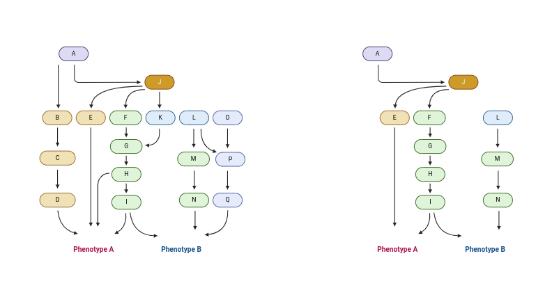
I implemented a PreProcess class that identifies and removes 3 types of reactions:
- Blocked reactions: cannot carry a flux in any condition.
- Zero-flux reactions: cannot carry a flux while maintaining at least 90% of the maximum growth rate.
- Metabolically less-efficient reactions: require a reduction in growth rate if used.
Example of using the reduce function of the PreProcess class on the E. coli core model:
cobra_model = load_json_model("ext_data/e_coli_core.json")

obj = PreProcess(cobra_model, tol = 1e-6, open_exchanges = False)

removed_reactions, reduced_dingo_model = obj.reduce(extend = False)
Explanation of the parameters and returned objects:
open_exchanges: A parameter for thefind_blocked_reactionsfunction of theCOBRApylibrary. It controls whether to open all exchange reactions to very high flux ranges.removed_reactions: A list that contains the names of the removed reactions.reduced_dingo_model: A reduced model with the bounds of removed reactions set to 0.
Users can choose to remove an additional set of reactions, by setting the extend parameter to True.
These reactions do not affect the value of the objective function, when removed.
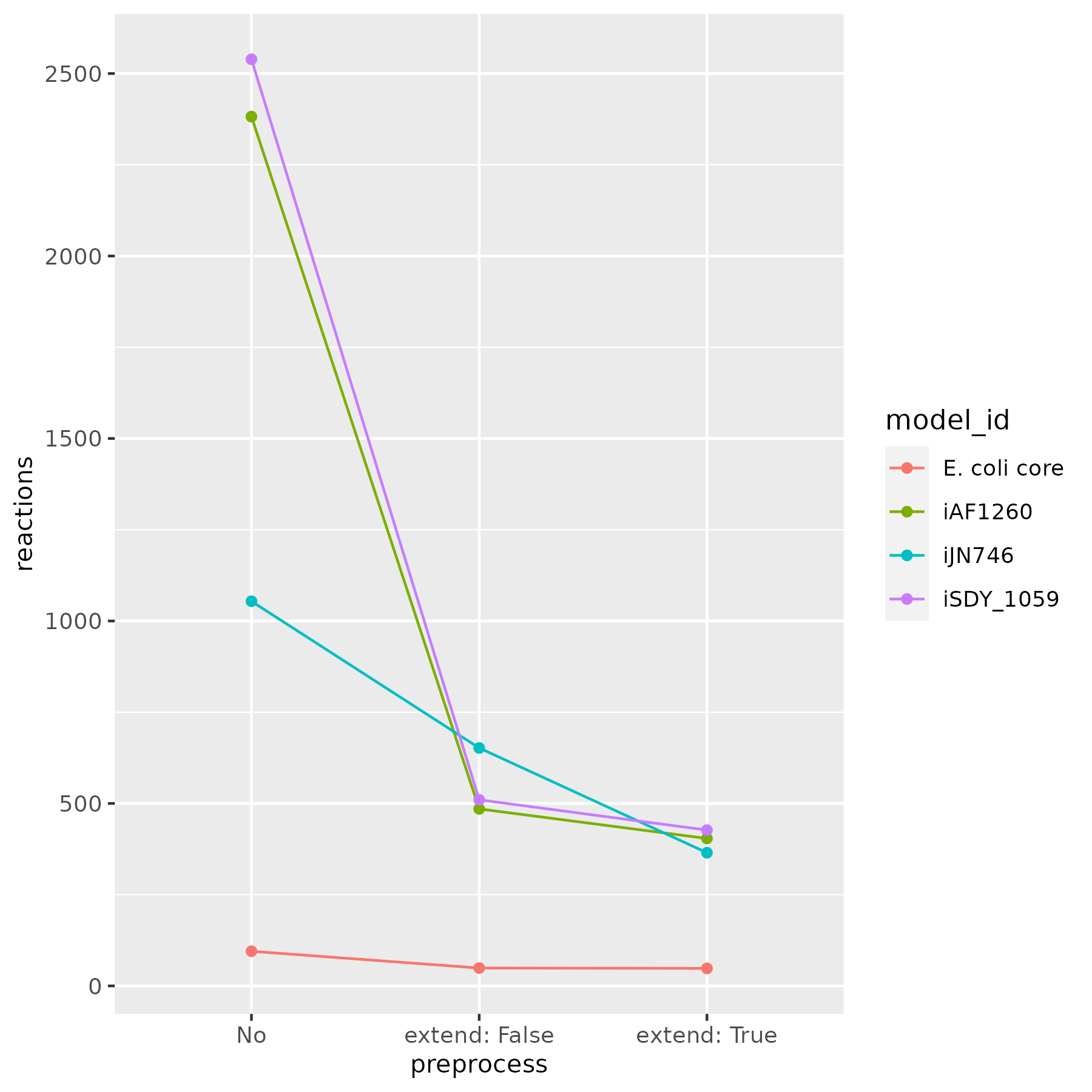
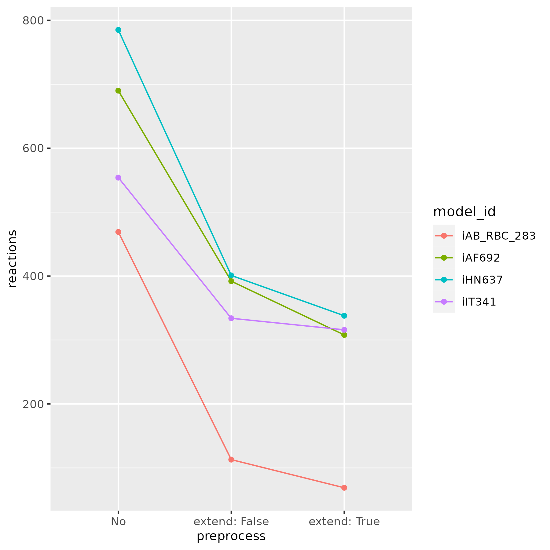
Reduction with the PreProcess class has been tested with various models [2], some of which are included in dingo’s [3] publication article too.
A figure below shows the number of remained reactions, after calling the reduce function with extend set both to False and True.
Note that when extend is set to True, the reduction is based on sampling, so slight changes in the number of remaining reactions may occur.
It is recommended to use extend set to False for large models due to higher computational time.
Correlated Reactions
- Reactions in biochemical pathways can be positively correlated, negatively correlated, or uncorrelated.
- Positive correlation: if reaction A is active, then reaction B is also active and vice versa.
- Negative correlation: if reaction A is active, then reaction B is inactive and vice versa.
- Zero correlation: The status of reaction A is independent of the status of reaction B and vice versa.
- These features are derived from the second pull request.
I implemented a correlated_reactions function that calculates reactions steady states using dingo’s PolytopeSampler class and creates a correlation matrix based on the pearson correlation coefficient between pairwise reactions.
This function also calculates a copula indicator to filter correlations greater than the pearson cutoff.
Example of using the correlated_reactions function on the E. coli core model:
dingo_model = MetabolicNetwork.from_json("ext_data/e_coli_core.json")

sampler = PolytopeSampler(dingo_model)
steady_states = sampler.generate_steady_states()

corr_matrix, indicator_dict = correlated_reactions(
                              steady_states,
                              pearson_cutoff = 0.99,
                              indicator_cutoff = 2,
                              cells = 10,
                              cop_coeff = 0.3,
                              lower_triangle = False)
Explanation of the parameters and returned objects:
steady_states: Reactions steady states returned from dingo’sgenerate_steady_statesfunction.pearson_cutoff: A cutoff to filter and replace all lower correlation values with 0.indicator_cutoff: A cutoff that corresponds to the copula’s indicator, filtering correlations greater than the pearson cutoff.cells: Defines the number of cells in the computed copulas.cop_coeff: Defines the width of the copula’s diagonal.lower_triangle: A boolean value that, whenTrue, keeps only the lower triangular matrix, useful for visualization.corr_matrix: The calculated correlation matrix with dimensions equal to the number of reactions of the given model.indicator_dict: A dictionary containing filtered reaction combinations with the pearson cutoff, alongside their copula indicator value and a classification for the correlation.
I also implemented a plot_corr_matrix function to visualize the correlation matrix as a heatmap plot.
In reduced models, there is an option to plot only the remaining reactions’ names if they are provided in a list.
Example of using the plot_corr_matrix function:
plot_corr_matrix(corr_matrix,
                 reactions,
                 format = "svg")
Explanation of the parameters:
corr_matrix: A correlation matrix produced from thecorrelated_reactionsfunction.reactions: A list of reaction names that will appear as labels on the heatmap axes.format: Defines the desired image saving format.
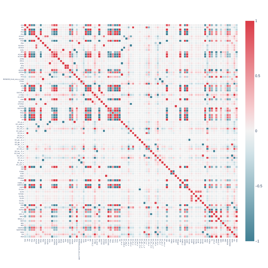
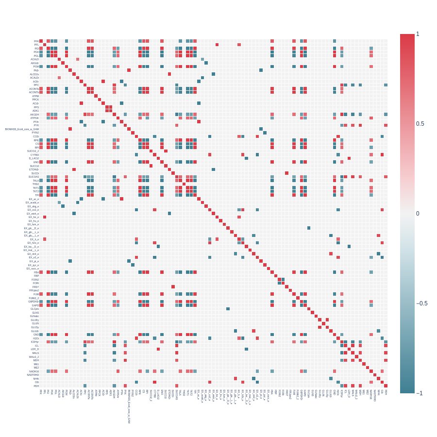
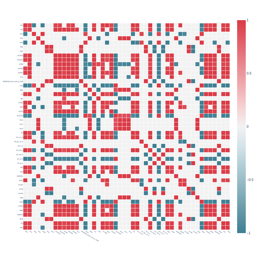
We will examine the capabilities of the correlated_reactions function using heatmap plots from the E. coli core model.
Heatmap from a symmetrical correlation matrix without pearson and indicator filtering:
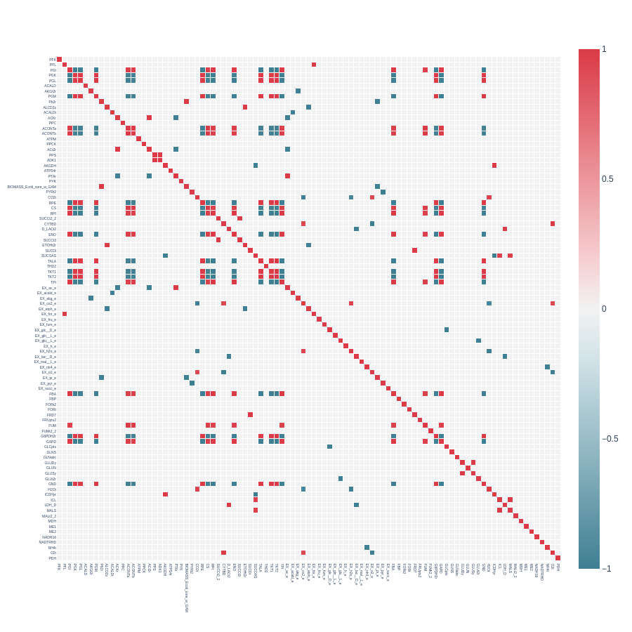
Heatmap from a symmetrical correlation matrix with pearson_cutoff = 0.7 and without indicator filtering:
Heatmap from a symmetrical correlation matrix with pearson_cutoff = 0.7 and with indicator_cutoff = 100:
Heatmap from a triangular correlation matrix with pearson_cutoff = 0.7 and with indicator_filtering = 100:
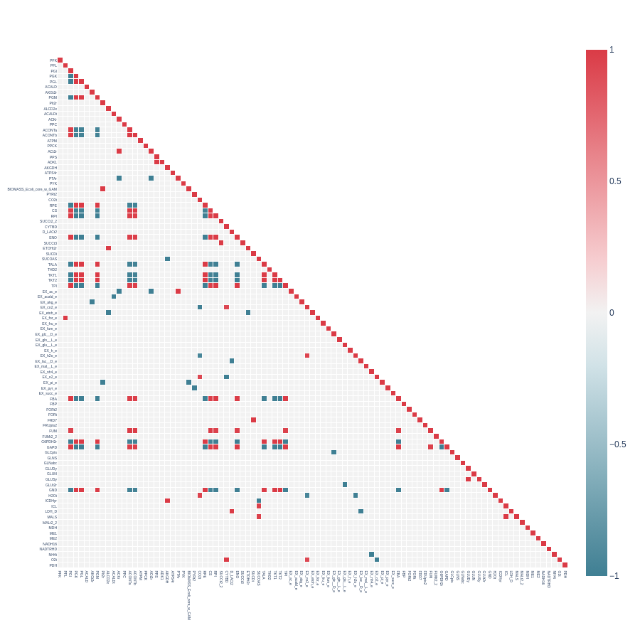
Now we will examine heatmap plots from reduced E. coli core models.
Heatmap from a symmetrical correlation matrix with pearson_cutoff = 0.7 and with indicator_filtering = 100, from a reduced E. coli core model with extend set to False:
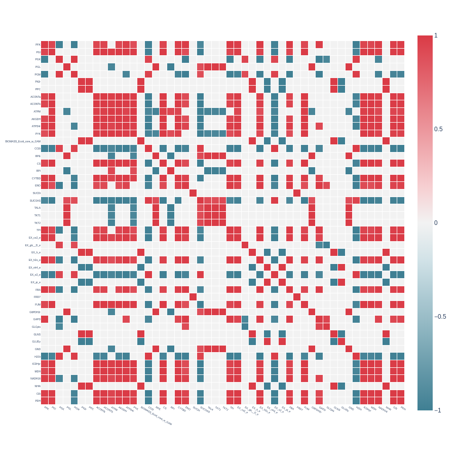
Heatmap from a symmetrical correlation matrix with pearson_cutoff = 0.7 and with indicator_filtering = 100, from a reduced E. coli core model with extend set to True:
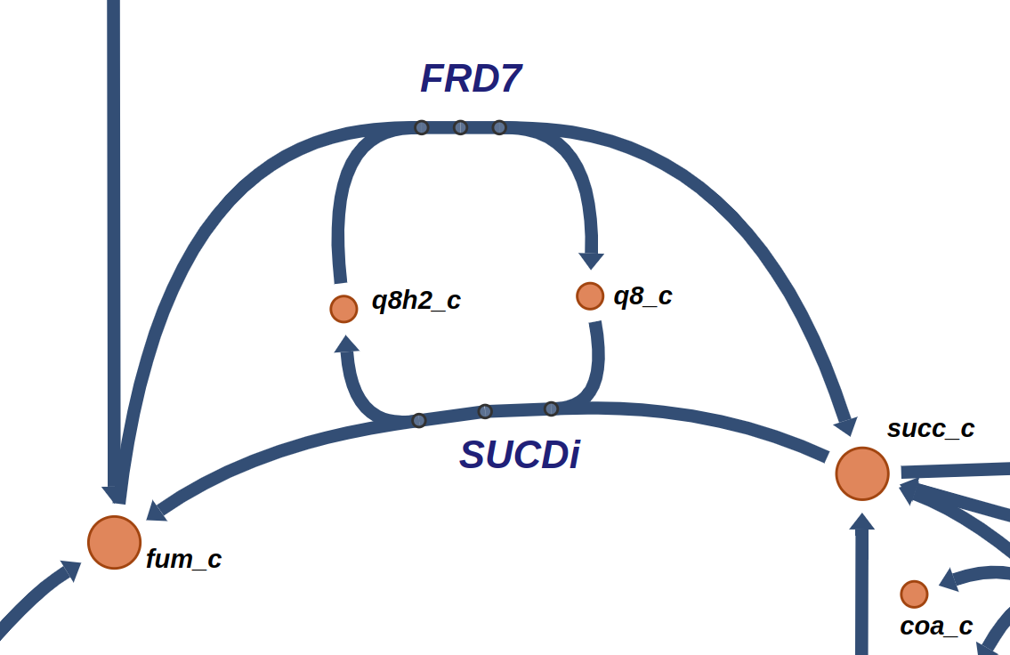
We observe that the additional reaction removed with extend set to True is FRD7, the least correlated across the matrix.
FRD7 is a fumarate reductase, appearing in a loop with SUCDi in the E. coli core model, as seen in the following figure obtained from ESCHER [4]:
Clustering
- Clustering based on a dissimilarity matrix reveals groups of reactions with similar correlation values.
- Reactions within the same cluster may contribute to the same pathways.
- These features are derived from the third pull request.
I implemented a cluster_corr_reactions function that takes a correlation matrix as input and calculates a dissimilarity matrix.
The dissimilarity matrix can be calculated in two ways: by subtracting each value from 1 or by subtracting each absolute value from 1.
Example of using the cluster_corr_reactions function:
dissimilarity_matrix, labels, clusters = cluster_corr_reactions(
                                         corr_matrix,
                                         reactions = reactions,
                                         linkage = "ward",
                                         t = 10.0,
                                         correction = True)
Explanation of the parameters and returned objects:
corr_matrix: A correlation matrix produced by thecorrelated_reactionsfunction.reactions: A list of reaction names.linkage: Defines the type of linkage (options:single,average,complete,ward).t: Defines a height threshold to cut the dendrogram and return the created clusters.correction: A boolean variable; ifTrue, the dissimilarity matrix is calculated by subtracting absolute values from 1.dissimilarity_matrix: A distance matrix created from the correlation matrix.labels: Index labels corresponding to a specific cluster.clusters: A nested list containing sublists of reactions within the same cluster.
I also implemented a plot_dendrogram function to plot a dendrogram from a dissimilarity matrix created by the cluster_corr_reactions function.
Example of calling the plot_dendrogram function:
plot_dendrogram(dissimilarity_matrix,
                reactions,
                plot_labels = True,
                t = 10.0,
                linkage = "ward")
Explanation of the parameters and returned objects:
dissimilarity_matrix: A distance matrix created by thecluster_corr_reactionsfunction.reactions: A list of reaction names.plot_labels: Specifies whether reaction names will appear on the x-axis.t: Defines a threshold to cut the dendrogram at a specific height, coloring the clusters accordingly.linkage: Defines the type of linkage (options:single,average,complete,ward).
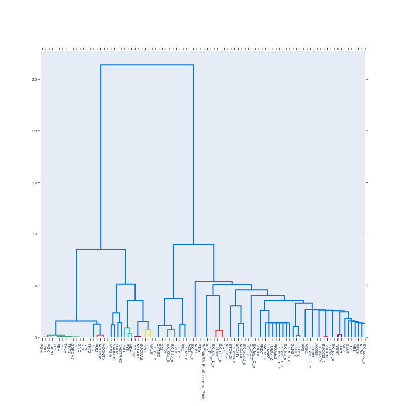
All dendrograms and graphs in this document are created from correlation matrices of the E. coli core model.
Dendrogram created from the plot_dendrogram function from a correlation matrix without pearson filtering and with correction = True:
Dendrogram from a correlation matrix with pearson_cutoff = 0.9999 and with correction = True:
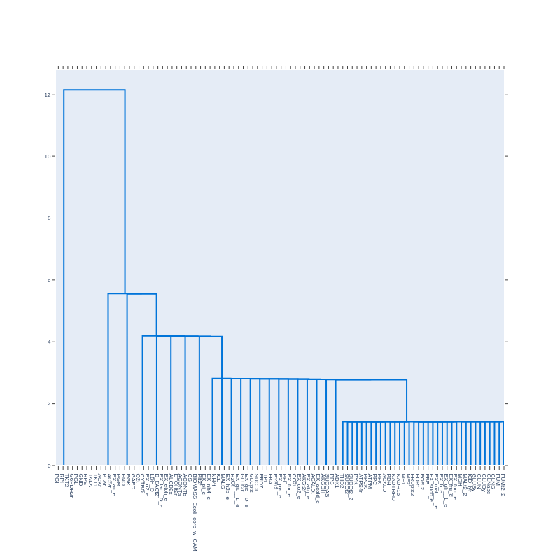
We observe distinct clusters. Graphs will reveal if these clusters interact with other clusters or reactions.
Graphs
- Creating graphs can reveal networks of correlated reactions, potentially corresponding to metabolic pathways.
- These features are derived from the third pull request.
I implemented a graph_corr_matrix function that takes a correlation matrix as input and creates network graphs.
This function also splits the initial graph into subgraphs.
Example of using the graph_corr_matrix function:
graphs, layouts = graph_corr_matrix(corr_matrix,
                                    reactions,
                                    correction = True,
                                    clusters = clusters)
Explanation of the parameters and returned objects:
corr_matrix: A correlation matrix produced by thecorrelated_reactionsfunction.reactions: A list of reaction names that will appear as nodes in the graphs.correction: A boolean value; ifTrue, it transforms the correlation matrix into the absolute correlation matrix.clusters: A nested list containing sublists of reactions within the same cluster, created by thecluster_corr_reactionsfunction.graphs: A list containing graph objects.layouts: A list containing graph layouts, each corresponding to a graph in thegraphslist.
I also implemented a plot_graph function to plot graphs given a graph object and its corresponding layout.
Example of using the plot_graph function:
plot_graph(graph, layout)
Explanation of the parameters:
graph: A graph object returned by thegraph_corr_matrixfunction.layout: A layout corresponding to the given graph object, also created by thegraph_corr_matrixfunction.
Example of calling the plot_graph function recursively for every subgraph returned:
for i in range(len(graphs)):
    graph = graphs[i]
    layout = layouts[i]
    plot_graph(graph, layout)
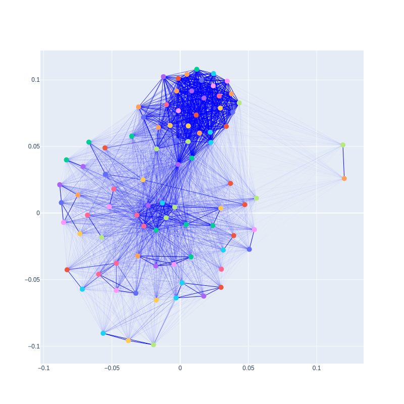
Graph created from the plot_graph function from a correlation matrix without pearson filtering and with correction = True:
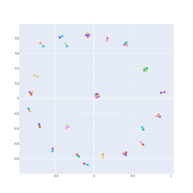
Graph created from a correlation matrix with pearson_cutoff = 0.9999 and with correction = True:
A subgraph created from a correlation matrix with pearson_cutoff = 0.9999 and with correction = True:
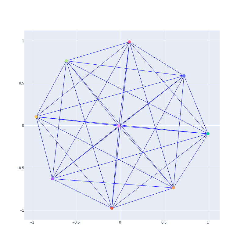
This subgraph has 9 nodes that correspond to 9 reactions close to each other in the topology of the E. coli core model.
These reactions are: PGI, G6PDH2R, PGL, GND, RPE, RPI, TKT1, TALA, TKT2.
Their topology can be seen in the figure below from ESCHER:
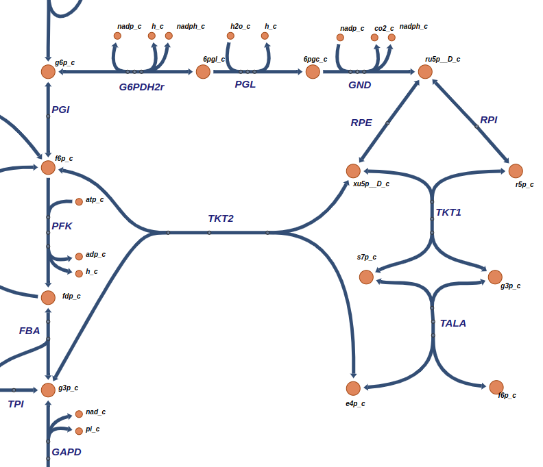
We can see that PGI seems to contribute to a different pathway. However it shares a common metabolite with G6PDH2r.
If we apply a stricter pearson cutoff (e.g., 0.99999), this reaction is removed from this subgraph, leaving only the remaining reactions.
This is an important observation: looser cutoffs lead to wider sets of connected reactions, forming larger metabolic pathways.
Conclusion
dingois a python package for the analysis of metabolic networks. I have expandeddingoby incorporating pre- and post- sampling features.- Flux sampling is an unbiased method that can advance research in metabolic models at both the strain and the community level.
- From model reduction to pathways prediction, the developed features incorporated into
dingodemonstrate the increased statistical value of flux sampling.
References
- [1] Adapted from “TNF pathway”, by BioRender.com (2024). Retrieved from https://app.biorender.com/biorender-templates
- [2] King, Z. A., Lu, J., Dräger, A., Miller, P., Federowicz, S., Lerman, J. A., Ebrahim, A., Palsson, B. O., & Lewis, N. E. (2015). BiGG Models: A platform for integrating, standardizing and sharing genome-scale models. Nucleic Acids Research, 44(D1), D515–D522. https://doi.org/10.1093/nar/gkv1049
- [3] Apostolos Chalkis, Vissarion Fisikopoulos, Tsigaridas, E., & Haris Zafeiropoulos. (2024). dingo: a Python package for metabolic flux sampling. Bioinformatics Advances, 4(1). https://doi.org/10.1093/bioadv/vbae037
- [4] King, Z. A., Dräger, A., Ebrahim, A., Sonnenschein, N., Lewis, N. E., & Palsson, B. O. (2015). Escher: A Web Application for Building, Sharing, and Embedding Data-Rich Visualizations of Biological Pathways. PLoS Computational Biology, 11(8), e1004321–e1004321. https://doi.org/10.1371/journal.pcbi.1004321